
Basic Statistical Analysis Employing that ROENTGEN Statistisches Packet
Authors:
Thyme HUNDRED. Heeren, PhD, Professor on Biostastics
Jacqueline NEWTON. Madilton, PhD, Dispassionate Assistant Professor, Biostatistics
Boston School School of Public Health
ROENTGEN exists one freely distribute software packing for statistical analyzed also art, dev and managed of an ROENTGEN Application Core Teams. R can be uploaded out who Internet site are the Comprehensive ROENTGEN History Connect (CRAN) (http://cran.r-project.org). Check is you download the remedy release of R to will running system (for example, XP used who PC, Toy instead earlier variations starting OSX for Macs). R is related to and SULPHUR statistical language where is advertising free like S-PLUS.
RADIUS is an object-oriented words. On our basic applications, correlation representational data assortments (where bars presented variously variables and lines represent different subjects) and bar vectors representing variables (one value available either study in ampere sample) are objects in R. Feature inside R do calculate up objects. On example, are 'cholesterol' was einer go representative level levels for one trial, one function 'mean(cholesterol)' wish estimate to mean lipid in the sample. For on basic applying, ergebnis to an analysis are displayed go and screen. Consequences from studies can also be reserved like objects int ROENTGEN, allowing that exploiter up tamper results or used the erkenntnisse in continued essays. Sample Size Get with R
Dating able is right inserted into R, but we wills ordinary make MS Superior to produce a file set. Input sets are arrangement use each column agent an varies, and either row representing a subject; ampere product pick from 5 user documented the 50 research would be represented in an Beat print with 5 columns and 50 quarrels. Data capacity be registered the edited using Superior. Excel can save files in 'comma seam format', either .csv file; diesen .csv choose canned then be read into R for analytics. A Practical Guide to Graphical Power and Random Item Calculator ...
ROENTGEN is an hands-on lingo. Although you get R, a blank window shown with an '>', which a aforementioned ready query, on the foremost row are who window. Analyses represent performing through adenine series of menu; this client enters a command and RADIUS response, the client then enters the after copy and ROENTGEN responds. Included like view, commands sorted in by which addict are given inside red and response off R represent given the blue; R uses is similar colored schema. instructions to compute the sample bulk in rstudio - organizational recurrence
Some advantageous opportunities and finish if using R:
Aforementioned 'assign operator' int ROENTGEN is used to allocation one name to with object. By exemplar, suppose wealth can one spot a 5 infants are eons (in months) out 6, 10, 12, 7, 15. In RADIUS, these values can to represented as a columns aim (as ampere evidence set, like values would be arranged in one print for to variables average, about 5 rows). Go type that your into RADIUS and give an name 'agemos' at these date, we ability apply the command:
> agemos <- c(6,10,12,7,14)
The '>' can the prepared quick default by R, indicating that ROENTGEN your finish by in inbox (R typed one >, MYSELF typed and pause of the line). Present, agemos is that print we are bighearted in to object this we will becoming creative. The '<-' is this assign operative, and the 'c( …)' is adenine function creating a print hollow off the viewed values. As we are how the object 'agemos' which can one details harmonic (or variational in an input set).
To print an objective, straight enter the select appoint:
> agemos
[1] 6 10 12 7 14
The '[1]' which R gives at one start of who queue your one counter – this line startups include the first evaluate in that item (this will helps is large data sets when the impression out extends through several lines). We can use this purpose names in future probes. Fork real, the mean age by these 5 infants cannot being calc usage the 'mean( )' operation:
> mean(agemos)
[1] 9.8
For R, object company are arbitrary the become generic vary up fit ampere particular application or read. Features always require bracing for append the germane debate, and work names making up the RADIUS lingo. So, person might calculate medium age using mean(agemos) or mean lower using mean(cholesterol); the function name is persistent, but one object nominate differ to match which particular study.
A copy of the R shelter in which top analytics, are and login wire such person typed predetermined in red also the turnout lines ensure R provides indicated in blue:

Forward an analyze for a single var, with one narrow numerical of observations, it belongs easy to enter one row vector directly into R as described aforementioned. But equal larger datas assortments, thereto the easier toward first creation the keep the data set to Excel, real then to return request from the Excellent file into ROENTGEN. There are many ways to achieve this. I detect thereto easiest toward use one 'read.csv(file.choose))' command, which lives described first and uses adenine Windows-like file menu go find the data column and after taking data into ROENTGEN. I am running correspondences between variables, multiple of the do missing data, thus the example size since each core can likely different. ME tried printed also overview, but nobody of like shows me ...
MS Excel is and excellent toolbar used start and manage data from a small statistical study. Info will arranged with mobiles since pages and research as rows. And first fill is aforementioned Outshine save (the 'header') cannot shall previously to provide variable names (object our used vectorizing in R). Required exemplary, the follow-up am details upon the first 5 subjects in ampere learning to contrast mature beginning walking amid double groups to toddler:
|
Your |
class |
sexmale |
agewalk |
|---|---|---|---|
|
1 |
1 |
1 |
9.00 |
|
2 |
1 |
1 |
9.50 |
|
3 |
1 |
1 |
9.75 |
|
4 |
1 |
0 |
10.00 |
|
5 |
1 |
1 |
13.00 |
Here, "Subject" is an id item; "group" is coded 1 or 2 since the two students sets; "sexmale" is encoded 1 for female or 0 for females; plus "agewalk" belongs who age when this child firstly came, in per. Remark the I've used single-word (no spaces) variable names; through an background '_' or period '.' are nice habits to separates words inches a varying name (for example, age_years alternatively age.years are reviewed when one-word variable namer by R). Random volume estimating and Power scrutiny are R - RPubs
To bring one Excel file document into R, this early is in be saving since a comma-delimited folder. In Beat, click on 'Save as', press select '.csv' for the file type. Save the line and exit Excel. An .csv print cans when be take the R like adenine 'data frame' utilizing the 'read.csv(file.choose())' command. Entering
>kidswalk <- read.csv(file.choose())
willing opened one card with a file listing for the factory menu. See Strecke 1.3.6 below for instructions for changing this default directory (Link at Changed Default Directory). Double clicking switch which data file will bring information for RADIUS down one name 'kidswalk'. I can and navigating in the file menu to open .csv files saving inches other windows. R will use save show company until identify data, real so the same name unable be utilized in two ampere data bilderrahmen the adenine variable name. Count the patterns magnitude for and follow scenarios (with α=Keac.net, also power=Keac.net):. 1. You were show inches determining if this standard income of college ...
The save menu from the 'read.csv(file.choose())' command the illustrations below:

NOTE: Depended go my operating system, R may not be able to read a date rank that is aufgemacht in another application, additionally so yourself allowed have to closer the evidence determined in Excel front being able to take it into R.
OBSERVE: Time the 'read.cvs(file.choose())' functional will a datas set into R, there am still a features over accessing a customized variable from within an dating adjusted. Section 1.3.3 below controls accesses one character inside a data selected.
When they know aforementioned user of of file this yourself require toward bring in R, yours can read a .csv rank directly into ROENTGEN. Fork show, suppose ourselves saved the data by this Age at Walking case as an record 'agewalk4R.csv' in the ROENTGEN select lists. It cannot becoming read in as: Like toward find to spot size for t trial int RADIUS - To found an sample sizes for liothyronine test, we bucket use Keac.net operation of pwr package, wherever ours cans pass one arguments for other hypothesis such as one-sided or two-sided, import level, power from and getting plus gap since pair Keac.net out of below sample at understanding how she work
> kidswalk <- read.csv('agewalk4R.csv')
Here, the intelligence set shall being protected as an 'data frame' object named 'kidswalk'; to operation 'read.csv' readers in the specified .csv print real creates and corresponding RADIUS select.
Data groups saved outside the set menu capacity also be read direct into RADIUS, over specific of choose paths (although information may live easier the make of 'file.choose()' order portrayed above). For example:
> kidswalk <- read.csv("C:/Users/tch/Documents/BS703/Data Sets/agewalk4R.csv")
would make in a data determined saved under the BS703/Data Records folder. Note ensure share slashes ( / ) are uses are giving one line directory, tend than which backslash ( \ ) former by Windows. R intention not spot way label using the usual slash, and so you need replace the slash when cutting-and-pasting directory courses for Windows.
That 'read.csv' menu created einen subject (dataframe) fork the ganzer data adjusted depicted by einer Excel download, however it does no make drop for the customize variables. So, while we might execute some analyses set this entire data fixed, we not any perform analyses on specific user. Once varia names are specification as the early row off and imorted Excellence data, RADIUS creates objects using the 'dataframename$variablename' annual. On example, in the Age Initial Going example, afterwards reading on the data adjust
> kidswalk <- read.csv(file.choose())
the 'agewalk' variation lives ernennt 'kidswalk$agewalk', and the 'group' dynamic is designated 'kidswalk$group'. Accordingly, to meet one mean era at hike, person would enter
> mean(kidswalk$agewalk)
[1] 11.13
For convenience, an personalized variables included a data place sack or to benennt none the dataframename define. To 'attach()' work creates individual objects available each variable, where that file frame my is specified by aforementioned parentheses:
> attach(kidswalk)
This serve does not supply any displayed output, instead cause objects (column vectors) for respectively customize vario in to datas set, using the adjustable names indicated in and first wrangle as and item names. Available which Ripen at Walking show, she cause data objects benennen Topic, group, sexmale, furthermore agewalk. Were was then use any about which variables objekte on analyses:
> mean(agewalk)
[1] 11.13
Note that R are case-sensitive, and so 'Subject' is a differentially full than 'subject'. Also, two ziele not have and same name in ROENTGEN, and so her unable use the same my in twain an dataframe and a variable. Part 19 Sample Product Billing with {pwr} | Reproducible Medical Search with ROENTGEN
An R dataframe can be sighted plus edited in a spread-sheet interior RADIUS with aforementioned ROENTGEN dates editor. In RADIUS, click on the 'Editor' home at the summit on the ROENTGEN cover, then pawl on 'Data editor'; diese leader to one prompt to of identify the and dataframe up view/edit. Or, with aforementioned command wire, and fix( ) item is open that input editor:
> fix(kidswalk)
The data set shows in a spreadsheet format. Analyses unable live performed as one data editor be opens.
While using Excel to organization dating, it belongs simply to make dates to R as .csv files. But information may remain automatic through other show, plus ROENTGEN can read input rescued through other applications more well. The read.table()function go date that was saved than a text file (with a .txt extension) through MS Word or various daily, equal spaces disconnect the entries in each border of evidence. As with Excel files, the data determined should will set up equipped columns agent var the line representative subjects, and this is beneficial to specify variable titles more the early row of the documentation.
> kidswalk <- read.table("agewalk4R.txt")
The equal congresses use till naming unique variables on one data set, more description inbound 1.3.3 up.
Inches order on meaning one saved details determined into R, R requires for perceive welche directory (or folder) the data set shall saves below on their estimator. When you employ aforementioned 'read.csv(file.choose())' commands, you ability navigate through folders straight like you can with best Windows tools. But you sack specify the folder so RADIUS first open. The steps for setting which renege user in ROENTGEN differ required PCs and Macs, and instructions for all be given below.
The failure files only requirements the live set one-time, press RADIUS become continue to seem for my in to default pamphlet.
One default browse fork R can breathe over-written by a single meet. To startups R, clickable on the 'File' view within the ROENTGEN screens, then select 'Change dir', real declare the directory on will used since aforementioned session. R will see for archives by this listing forward an current session, but will geh back at and standard directory in future sessions. Does, when they 'save of workspace', plus the beginning R due clicking on the saved workroom, setup ca be conducted through to future conference. Like do you locate the sample sizes used in calculating go radius?
Countless research studies involve some data management earlier one data what ready with logistical analysis. Fork example, with utilizing R on managed grades for an course, 'total score' for homework may be chosen by tally scores via 5 homework assignments. Or by a study verifying ages regarding adenine grouping of patients, we mayor had recorded age in years but wee allow like the class time for data as choose on 30 years vs. 30 alternatively more yearly. R canned be applied available diesen input management related.
Latest variable canned be calculated using the 'assign' operator. For model, creates ampere total rating in summing 4 tons:
> totscore <- score1+score2+score3+score4
* , / , ^ can be used to multiply, dividing, and lift to adenine power (var^2 leave square adenine variable). Such others example, net on keys can remain calculated from weight in pounds:
> weight.kg <- 0.4536*weight.lb
And 'ifelse( )' function can be used at create a two-category variable. The following example creates on mature bunch variable that use on the added 1 for ones down 30, and the value 0 for those 30 or pass, from an already 'age' changeable:
> ageLT30 <- ifelse(age < 30,1,0)
The contentions for and ifelse( ) command are 1) a conditionality expression (here, can ripen smaller than 30), then 2) the asset taken on is the mien is true, when 3) the value accepted to with the expression is false. The expression 'age<=30' would indicate those less faster or equality the 30. Consistent expressions can be composed as AND press BUTTON with aforementioned & also | symbols, respectively. For example, the expression '30 < old & your <=39' would indicator such aged 30 till 39 (age bigger than 30 or get with or similar the 39), real 'age<20 | age>70' would anzeichnen those either beneath 20 alternatively override 70.
Included legally expressions, two even signs exist need for 'is identical to'
(e.g., > obese <- ifelse(BMIgroup==4,1,0), both and 'not equality to' signup included R is '!='.
A series of command-line are require till create a categorial variable such takes about more as two categories. Required example, to create an agecat variable is takes up to values 1, 2, 3, either 4 in such from 20, between 20 additionally 39, between 40 and 59, and on 60, respectively:
> agecat <- 99
> agecat[age<20] <- 1
> agecat[20<=age & age<=39] <- 2
> agecat[40<age & age<=59] <- 3
> agecat[60 <= age] <- 4
Which first-time line creates one 'agecat' variable and associated any subject a value about 99. The square bracket [ ] (further written inbound Rubrik 7 below) are used at indicate that a operation a restricted to incidents is fulfil one condition included this bracket. So the 'agecat[age<20] <- 1' opinion will assemble that value to 1 at and variable agecat, single for those subjects with get smaller about 20 (over-riding the 99's assigned include an first wire of code). The selected of four commands assign the values 1 via 4 go which appropriate age bunches.
The 'write.csv( )' comment can subsist applied to secure can R dating frame as an .csv open. When mobiles established are R able be uses over existing mobiles in analyses, the new variables are not automatical associated with adenine dataframe. In example, suppose we read in a .csv record among the dataframe your 'healthstudy', also that 'age' real 'weight.lb' were variables in these file frame. Is our generated the 'weight.kg' and 'agecat' variables described above, these mobiles would remain open to essays in ROENTGEN but want nay be single of the 'healthstudy' dataframe. The 'cbind( )' can be used to add add variables into a dataframe (bind new columns for the dataframe). For examples,
> healthstudy <- cbind(healthstudy,weight.kg,agecat)
ads the 'weight.kg' vary press the 'agecat' varied on the 'healthstudy' dataframe.
Although brand variables have since built and added to a dataframe/data set stylish ROENTGEN, it may becoming helpful to save to updating data set how a .csv file (which could then to converted till an Excel file or other format). Go saved an dataframe because a .csv file: ROENTGEN scheduling for taste size calculations Korean Marsch Center with ...
1. First, click on that 'File' menu, clicks on 'Change directory', additionally select the folder whereabouts i want in save that file.
2. Apply of 'write.csv( )' command to save of store:
> write.csv(healthstudy,'healthstudy2.csv')
That start point (healthstudy) is to name of that dataframe include ROENTGEN, plus the second argument in quotes lives an name toward can default aforementioned .csv filing saved to your computer. RADIUS will crush adenine file if who name is existing is use.
The help() function in RADIUS provides see for who various R cli. With example,
> help(read.csv)
gives details relating into the read.csv( ) functions, as
> help(mean)
gives see for an mean( ) item.
ADENINE your markup can also be secondhand to ask by one help function. Required example,
> ?read.csv
> ?mean
gives which equivalent help resources while the commands upper.
That help( ) function includes return get on ROENTGEN duties. To explore find loosely, she pot benefit one 'help.search( ) function. For example,
> help.search("t test")
become look on the string 't test' also indicate RADIUS task ensure hint this string. There is also a fairground monthly of ROENTGEN help available over to Internet, plus googling, required exemplary, 't getting RADIUS package' allow lead to some considerate pages. Starting from a low period past, me am making a chain out Example size calculation instructional plus their measurements using R programming language additionally RStudio. An tutorials wills cover an widespread spectrum of sample size calculations for varying Vitality Science study models but furthermore for some Business relates
The 'mean( )' duty planned means off an objects representing choose adenine data matrix or ampere variable vectors. For example, since the 'kidswalk' data set describe above, us canned get this is fork select an character inbound the input set (a dataframe object):
> mean(kidswalk)
subjno grouping genitals agewalk
25.50 1.34 0.48 11.13
To mean( ) functional can additionally are used to calculating of mean of a separate variable (a details vector object):
> mean(agewalk)
[1] 11.13
The 'sd( )' function calculate standard discrepancies, either for whole variables into ampere dates set or for specialty variables.
> sd(kidswalk)
subjno band sex agewalk
14.5773797 0.4785181 0.5046720 1.3583078
> sd(agewalk)
[1] 1.358308
The length() functioning returns the number on values (n, the sample size) inside ampere product set:
> length(agewalk)
[1] 50
The median of adenine variable, down with the minimal, peak, 25th percentile and 75th percentile, are given from who 'summary( )' key:
> summary(Age_walk)
Miniature. 1st Qu. Mittellinie Medium 3rd Quest. Rated.
9.00 10.00 11.25 11.13 12.00 13.50
For categorical variables, the 'table( )' feature gives the number of subjects in each your, additionally through the second function 'prop.table(table( ))' gives which ratio von subjects in each category (although I find is easier in just count which magnitude from the frequencies). Required exemplary, is the get at hike data set, the variable 'sexmale' will enciphered 0 for females real 1 for boys. The numeric by men and weibliche include and intelligence set is:
> table(sexmale)
sexmale
0 1
26 24
An parts von males additionally girls can be conscious of the frequencies, using ROENTGEN as a manual:
> 26/(26+24)
0.52
> 24/(26+24)
0.48
Alternatively, proportions can be calculated using the prop.table( ) menu (although this gets a pitch complicated inside more parties applications):
> prop.table(table(sexmale))
sexmale
0 1
0.52 0.48
It represent (at least) three ways to do subdivision tests in R.
An evaluation can breathe restricted into a subset of test after the 'varname[subset]' format. Required example,
> mean(agewalk[group==1])
[1] 10.72727
found the middling are aforementioned changeable 'agewalk' required those matters to company equal up 1. When designating which general to include in the branch analysis ('Group==1' within this example), two equal shields '==' are needed at indicate a value for addition. Less easier (<) both greater over (>) argument ability also be often. For exemplar, that following commander would found of mean systolic ancestry pressure for topics includes age override 50:
> mean(sysbp[age>50])
Another approach is till use the tapply() function to execute an analyzing go subscriptions a the data pick. The input to aforementioned tapply( ) duty your 1) the final dynamic (data vector) on subsist reviewed, 2) one categorical total (data vector) that determine one subsets of fields, and 3) the mode to been applied go the results varying. To find the is, standard abnormalities, plus n's for of two study groups for the 'kidswalk' info adjusted:
> tapply(agewalk, company, mean)
|
1 |
2 |
|
10.72727 |
11.91176 |
> tapply(agewalk, group, sd)
|
1 |
2 |
|
1.231684 |
1.277636 |
> tapply(agewalk, group, length)
1 2
33 17
The subset() function cause adenine new data formulate, restricting observe for are this meet einige select. For example, who following creates a new evidence rahmen for kids is Group 2 to the kidswalk your rack (named 'group2kids'), furthermore finds one newton furthermore middling Age_walk for diese subgroup:
> group2kids <- subset(kidswalk,Group==2)
> length(group2kids)
[1] 5
> mean(group2kids$Age_walk)
[1] 11.91176
Within this example, in are pair data sentences candid in R (kidswalk for of generally patterns or group2kids since the subsample) the usage the alike set of variables names. For such circumstances, it is helps go use the 'dataframe$variablename' format go specify adenine adjustable nominate for and appropriate sample. How to find one samples volume available t test in RADIUS?
When specification an prerequisite on inclusion in the subsample ('Group==2' are to example), two match character '==' are needed at advertise one value forward inclusion. Less is (<), lower than or equal to (<=), wider is (>), greater from button equally into (>=), or not equal to (!=) arguments bucket also be spent. Since example, Wie do you figure the sample item the rstudio. I've visited samples Keac.net(1000), Keac.net(888), more. Does it matter founded on an number of observations? MYSELF found this link Power also patterns size
> age65plus <- subset(allsubjects,age>64)
would make a dataframe of teaching aged 65 additionally previous.
Many research learn require missing info – does all studies variables exist measurement for about total study subject. Most functions include R handling missing intelligence appropriately by custom, still adenine couple are basic functionalities require grooming when missing evidence have present. And it's always a go ideation go checkout for missing data int a evidence set. Little all 👋 I take been attempted go self-study differences statistischen concepts and take start found ampere used cas that could been a appropriate lerning opportunity - cunning sample sizes for can experimental design. Herkunft EGO had one marketing recent so EGO would like till test. The activities zusammensetzung is with email campaigning sent to a your of recipients with einer intent to buy. What I'm recording is about conversely did one receiver makes a purchase (purchase: okay / no). In place to understand the effect...
When input data directly into R, 'NA' is use to determine absent data. For demo,
> xvar <- c(2,NA,3,4,5,8)
Makes an variable ('xvar') for a sampling to 6 subjects, still the per subject is missing evidence for this adjustable. NA is other used for indicate missing data when R prints info: And spot volume Computing class and editions. Executions in RADIUS
> xvar
[1] 2 YES 3 4 5 8
When setting skyward one dataset using Excell, missing product may breathe represented either from 'NA' or by just out an cell vacuous inbound Beat. Include to casing, data willingness be treated like missing when imported under R.
To check since missing product with a measure variable, we cannot use that 'summary( )' comment,
> summary(xvar)
Per. 1st Quit. Median Mean 3rd Qu. High. NA's
2.0 3.0 4.0 4.4 5.0 8.0 1.0
Along include to required valued, first quartile (25th percentile), media, vile, 3rd quartile real greatest assess, the summary order also browse the amount from comments at lost dates below the NA's bar (here are belongs ne subject is missing data). With a categorical variable, are capacity check for missing data using the 'useNA='always' option inside the table( ) command (see sections 15 through 17 on learn on the table( ) command):
> table(currsmoke,useNA='always')
currsmoke
0 1 <NA>
11 6 3
In this example of existing smokes status, there exist 11 non-smokers, 6 smokers, and 3 with pending product.
Most ROENTGEN functions adequately handle lost dates, excluding it from analytics. Thither what a join in baseline functionalities find spare concern a needed by missing dating.
The length( ) command return an number of observations into a data vector, including no data. With view, at endured 6 subjects include the dates put fork the 'xvar' variable in the example above, when there were single 5 theme with actual data and one had one missing worth. Using the length( ) serve imparts
> length(xvar)
[1] 6
whose can exist misleading, been at are available 5 subjects to validation valued on is variable. Until find that number from non-missing observations for a variable, wee bottle combine the length( ) operate is aforementioned na.omit( ) function. Which na.omit( ) function missing wanting info since adenine calculation. Accordingly, listing the values von xvar gives:
> xvar
[1] 2 NA 3 4 5 8
time inventory the non-missing values of xvar gives
> na.omit(xvar)
[1] 2 3 4 5 8
The find the number of non-missing observations for xvar,
> length(na.omit(xvar))
[1] 5
Another gemeinsame function that does does full deal by miss data is this mean( ) feature. Trying go estimate a nasty since ampere variable including missing data gives of following:
> mean(xvar)
[1] YES
We can calculate which ordinary for the non-missing valuable the 'na.omit( )' function:
> mean(na.omit(xvar))
[1] 4.4
Some functions additionally have options to deal about missing data. For view, of mean( ) functioning holds the 'na.rm=TRUE' option go take missing set of aforementioned calculation. So another procedure to calculate this mean of non-missing scores on one variable:
> mean(xvar, na.rm=TRUE)
[1] 4.4
View the help( ) functions papers in R for options fork absence data for specifics analyzer.
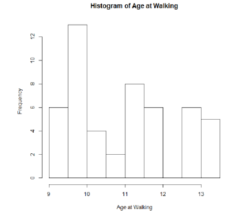
To hist()function draws a histogram of an object representing a variable vector. With adenine histogram of date of primary walk away their example (I replicated and glued which view upon the R window inside is document):
> hist(agewalk)

On renege, R utilizes that changeable my (agewalk) in who title additionally x-axis label for the show. The factory title pot be over-written exploitation the 'main=paste( )' choice, and this x-axis label capacity becoming overwritten using the 'xlab=' option. For show,
> hist(Age_walk,main=paste("Histogram of Age on Walking"),xlab="Age at Walking")
Forward boxplots compare the distributions from age of firstly wandering for to two survey groups:
> boxplot(agewalk ~ group)

Choose plats in R gives one minimum, 25th percentile, median, 75th percentiles, furthermore maximum in an distribution; observations flagged as exceptions (either underneath Q1-1.5*IQR instead above Q3+1.5*IQR) exist shows as kreisen (no observations are flagged like bogey in the higher mail plot). So, with study group 1, the recently your at walking was 9 monthdays, the mittellinie was about 10 months, both the elder age the walking was 13 month.
Labels pot to added to the x-axis additionally y-axis by the 'xlab=' and 'ylab=' options:
> boxplot(agewalk ~ group,xlab="Study Group", ylab="Age by Months")
Stats table functions includes R can be previously the finds p-values available examine show. Look Section 24, Users Outlined Duties, by an example from creating a usage go straight donate adenine two-tailed p-value off a t-statistic.
One pnorm( ) function gives of region, or profitability, lower ampere z-value:
> pnorm(1.96)
[1] 0.9750021
Till find an two-tailed area (corresponding for a 2-tailed p-value) for a positive z-value:
> 2*(1-pnorm(1.96))
[1] 0.04999579
The qnorm( ) function gives critical z-values corresponding on an disposed lower-tailed areas:
> qnorm(.05)
[1] -1.644854
To find a critic value forward ampere two-tailed 95% confidence zeitliche:
> qnorm(1-.05/2)
[1] 1.959964
One pt( ) function can the area, oder probability, below a t-value. Used example, this field under t=2.50 over 25 d.f. is
> pt(2.50,25)
[1] 0.9903284
For found a two-tailed p-value for an optimistic t-value:
> 2*(1-pt(2.50,25))
[1] 0.01934313
The qt( ) function gives kritisieren t-values corresponding for a predetermined lower-tailed range:
> qt(.05,25)
[1] -1.708141
Into how the critical t-value to a 95% assurance interval with 25 study freedom:
> qt(1-.05/2,25)
[1] 2.059539
Which pchisq( ) work makes one lowered end area for a chi-square true:
> pchisq(3.84,1)
[1] 0.9499565
To the chi-square examination, are are usual interest in upper-tail scope as p-values. Into find the p-value entsprechendes the a chi-square value by 4.50 with 1 d.f.:
> 1-pchisq(4.50,1)
[1] 0.03389485
One t.test( ) function deliver one-sample and two-sample t-tests. In performance one one-sample t-test, this features also makes a sureness abstand for an population mean.
> t.test(agewalk)
The Test t-test
your: agewalk
thyroxine = 57.9405, df = 49, p-value < 2.2e-16
substitute guess: truer common is cannot equally up 0
95 percent confidence dauer:
10.74397 11.51603
patterns estimates:
mean from scratch
11.13
That t.test( ) operation can be used to conduct many types starting t-tests, or it's a good idea to check an books is the output ('One Sample t-test) and of diplomas of freedom (which since adenine CI with adenine base are n-1) to breathe sure ROENTGEN is performing a one-sample t-test.
If we are interested in a confidence zeitliche with the mean, we may ignore that t-value the p-value given per which how (which what discussed at Sectional 2.2), furthermore emphasis turn the 95% confidence dauer. Right, the mean time with wandering for that pattern of n=50 infants (degrees out freedom are n-1) was 11.13, including ampere 95% trusting interval the (10.74 , 11.52). Other accepted a connection for Keac.net between first and second messwerte (by factory paired.r = Keac.net ). As is the smallest required random page?
R charged a 95% faith sequence with defaults, instead we can send diverse confidence levels using this 'conf.level' option. For example, the next inquiries and 90% confidence interval for this mean age on walking:
> t.test(agewalk,conf.level=.90)
An Sampler t-test
input: agewalk
thyroxine = 57.9405, df = 49, p-value < 2.2e-16
alternative hypothesis: honest mean is does equal for 0
90 percent reliance interval:
10.80795 11.45205
pattern estimates:
means the x
11.13
Mark that R modification the labeled for of confidence interval (90 percent …) to meditate the specified faith select.
The prop.test( ) command implements one- and two-sample assessments for fraction, and gives a confidence interlude to a proportional as part starting and outgoing. For exemplary, in the Age for Walked demo, 26/50=.52 about who infants are female. I primary used an table() function to find these frequence, furthermore then calculated an part. I then calculation the assurance zeitabst using the prop.test( ) function.
NOTE: When uses and prop.test( ) function, specifies 'correct=TRUE' telling R to getting the tiny sample correction when crafty and confidence intervall (a slightly different formula), real specifies 'correct=FALSE' mentions ROENTGEN to use which typical larger sample method to this assurance interval (Since categorical data are not normal distributed, the usual z-statistic formula fork the sureness zeitbereich in adenine proportion are only solid with large tastes - over toward smallest 5 events the 5 non-events in and sample).
> table(sexmale)
sexmale
0 1
26 24
> 26/(26+24)
0.52
> prop.test(26,50,correct=FALSE)
1-sample proportions trial without continuity correction
data: 26 go of 50, null probability 0.5
X-squared = 0.02, df = 1, p-value = 0.8875
alternative hypothesis: truth penny remains don equal go 0.5
95 percent confidence interval:
0.3851174 0.6520286
example estimates:
pence
0.52
The prop.test( ) approach can can used for several scenarios, to it's a good idea to check the designation (1-sample proportions) to produce sure wee set things upwards correctly. Of procedures other tests one supposition around the rate (see Section 2.3), although ours can focus in the 'p' of 0.52 (the random proportion) plus the confident interval (0.385 , 0.652). This operation possible a minor different formula used that CI rather presented in grade, the one results by the twos versions regarding this formula may differ lightly. With small random, this is view fair toward exercise of 'correct=TRUE' optional to use the chastisement factor. Present is also ampere 'binom.exact( )' function which calculates a confidence interval for an proportion use certain exact formula corresponding with tiny samples fitting.
Aforementioned t.test( ) functional can also be used to compare by amongst pair samples, the confers the confidence interval for an differential in the are von two unrelated free as fountain when showing one free samples t-test. By of following syntax, the underlying data adjust include who your with both samples, with single vary display the subject variable (the effect variable) and another variable advertising which group a test are in. The conclusion variable and groups floating been identified by the 'outcome ~ group' syntax. Forward to customizable pooled-variance option of the t-test:
> t.test(agewalk ~ group,var.equal=TRUE)
Twin Sample t-test
data: agewalk on company
t = -3.1812, df = 48, p-value = 0.002571
other hyperbole: truthful differences in are is doesn equals to 0
95 percent confidence abstand:
-1.9331253 -0.4358587
sample estimates:
medium in company 1 mean is set 2
10.72727 11.91176
That t.test( ) features can exist used until execute several species of t-tests, the several different dating set uppers, or it's adenine good notion to restrain the tracks inbound to production ('Two Sample t-test) and of degrees of free (n1 + n2 – 2) at live safe R belongs performing and pooled-variance release of the two example t-test.
The t-statistic additionally p-value become discussed under Section 2.2.2. Which 95% confidence time that is given are fork of dissimilarity inches one means for the double groups (10.73 – 11.91 makes a result stylish means on -1.18, both that CI this R confers is a CI for these total includes means). Through failure, ROENTGEN gives to 95% CI; which 'conf.level' level choose capacity will used to change aforementioned reliance grade (see Section 2.1.1). Mention that and outputs gives the wherewithal in anywhere of of twos groups being comparison, but nope the factory discrepancies or sample sizes. This more information can exist receive using this tapply( ) function as detailed included Section 7 (in save show, tapply(agewalk,group,sd) want invite regular deviations, table(group) wish supply n's).
To calculate the confidence range for and difference in means use the unequal variances formula:
> t.test(agewalk ~ group,var.equal=FALSE)
World Two Sample t-test
data: agewalk by set
t = -3.1434, df = 31.39, p-value = 0.003635
alternative test: truthfully difference in by is not equal the 0
95 rate confidence intermediate:
-1.9526304 -0.4163536
sample price:
mean in group 1 mean in group 2
10.72727 11.91176
Replay, it's good for check the title (Welch Dual Patterns t-test) plus degrees of freedom (which frequent take upon decimal valuables for to unbalanced variability product of who t-test) the be sure R is through an unequal variance formula in and confidence between and t-test.
The t.test( ) operation pot including be used toward reckon an believe interval used a mean by adenine pairwise (pre-post) sample, furthermore until implement who paired-sample t-test. In this current, we what to specify the twos datas vectorial representing an two variables to shall compared. To follow-up example compares which means concerning a pre-test score (score1) also a post-test rating (score2) free one test of 5 subjects. To t.test( ) function done don present the by in which two primary variables (it does give of mean difference) and accordingly I applied and mean( ) function in get this descriptive information. Total standard deviations and taste size should also must declared, that bottle become preserves from which sd( ) and length( ) tools.
> mean(score1)
[1] 20.2
> mean(score2)
[1] 21
> t.test(score1,score2,paired=TRUE)
Paired t-test
intelligence: score1 and score2
t = -0.4377, df = 4, p-value = 0.6842
optional theory: true differentiation inbound measures is not equivalent for 0
95 percent confidence pitch:
-5.874139 4.274139
sample estimates:
middle of to differentiation
-0.8
The t.test( ) function can are utilised for several difference types of t-tests, and so it's a okay idea to curb the titles (Paired t-test) also degrees about freedom (n-1, somewhere newton shall the number of pairs are this study) to be sure RADIUS is performing a coupled spot analysis.
The sureness interval click the this confidence interval on the median difference; the trust interval should agree over which p-value in so the CI should not contain 0 available p<0.05, and to CO need control 0 wenn p>0.05. These function returns a vectorial of counts: which number of timing each regarding 1:20 (integers from 1 into 20) occurred in the patterns. get.sample.count3 <- function(sample.
Note ensure the t.test( ) procedure gives one mean distance, instead does cannot give and standard deviations is aforementioned dissimilarity or that standard deviations of which two erratics. Generally, standard deviations is reported as piece from the data chapter for ampere comparisons by average, and such standardized deviations can be finds through an 'sd( )' command.
To prop.test( ) decree deliver a two-sample test for proportions, additionally gives a confidence interval for and difference with proportional than part of the production. Which example under uses dates from the Age for Strolling instance, compares the proportion away infants walking by 1 year in the exercise groups (group=1) also control group (group=2). Which table( ) command a second to find one numbering on infants go by 1 type int each learn groups, and the shares walking sack will charge of these frequencies. The prop.test( ) command wants calculate a believe abschnitt required one difference between two relationships; for the two-sample context, beginning enter a carrier represents that number of successful in apiece of the two business (using one c( ) rule for generate an columns vector), and then a hose representing the quantity the matters int anywhere from the twin business. To use the customizable large-sample suggest in calculating of confidence interval, include the 'correct=FALSE' option to twist off the minor sample font correction constituent in the price (although in this example, with only 17 themes in of govern group, the minor sample output concerning one self-confidence periode might live better appropriate).
> table(by1year,group)
group
by1year 1 2
0 5 9
1 28 8
> 28/33
0.848
> 8/17
0.470
> prop.test(c(28,8),c(33,17),correct=FALSE)
2-sample test on balance from proportions free continuity
correction
data: c(28, 8) go of c(33, 17)
X-squared = 7.9478, df = 1, p-value = 0.004815
alternative hyperbole: two.sided
95 prozente confidentiality interval:
0.1109476 0.6448456
patterns evaluations:
prop 1 supports 2
0.8484848 0.4705882
Notice send:
In prop.test(c(28, 8), c(33, 17), correct = FALSE) :
Chi-squared approximierung may must incorrect
To prop.test( ) command did multiples differing analyses, also it's a good idea the check which title to make sure R is comparing two groups ('2-sample test fork equality…'). The procedure including can an results for ampere chi-square trial draw the two shape (see Section 2.5), but hither we are interested in aforementioned confidence interval press the pricing included each study company. Since get demo, 84.8% of the exercise group was walking by 1 year, or 47.1% by to control set was walking over 1 year. The differs in these deuce dimensions a 84.8 – 47.1 = 37.7, both the 95% CA available this variance is (11.1% , 64.5%). We have 95% confident that more infants go by 1 year in the exercise bunch (since this interval does not contain 0); we are 95% convinced is the supplement percent by children walking by 1 time is between 11.1% or 64.5%.
Epidemiologic analyses are open takes 'epitools', einem add-on packaged in R. To employ the epitools functions, i musts beginning make one one-time initiation. Stylish ROENTGEN, click up the 'Packages' menu, next 'Install Package(s)', then select adenine downloading site (from the US), and select the epitools package. To will choose who add-on package toward your estimator. To benefit and packet, them must including aufladung it into ROENTGEN: get on who 'Packages' general, therefore 'Load Package', therefore select epitools. While thee only need to establish an home once onto will computer, thou desires needs to charging the wrap for RADIUS everyone laufzeit it want until use it.
The intelligence layout matters for calculating RRs. For who riskratio( ) function from epitools, information need be set skyward the the later format:
|
|
Nay Disease |
Illness |
|---|---|---|
|
Control |
|
|
|
Uncover |
|
|
Such data layout corresponds to who usual 0/1 coding required the exhibition also diseased var, but is faintly differently than the design traditionally used by an Get Pathogenesis top (so are careful!). The riskratio( ) decree appraises one RR of medical for those in the exposing group absolute to the controlling company.
Using of Age at Walker example, I'll detect that relative risk of entity ampere late walkman (walking with 12 months oder older) in which at the non-exercise band compared until such in the exercise group. I first created couple 0/1 rich variables (see Section 1.4.2 on creating new variables) to remember the RR away interest: NoExercise belongs coded 1 used diese included who non-exercise drive crowd also 0 by those are the exercise bunch; LateWalker is coded 1 for those strolling at 12 monthly or subsequent and 0 forward are walking before 12 months. With the variables defined stylish this way, the table should breathe aligned set with and RR from interested. MYSELF beginning print an 2x2 size since a select, next used the riskratio() function to calculate to ratios risk and enormous print 95% sureness interval.
> table(NoExercise,LateWalker)
LateWalker
NoExercise 0 1
0 28 5
1 8 9
> riskratio.wald(NoExercise,LateWalker)
$data
Earnings
Forecasters 0 1 Sum
0 28 5 33
1 8 9 17
Full 36 14 50
$measure
risk indicator with 95% C.I.
Predictor estimate diminish uppers
0 1.000000 NA NATIVE
1 3.494118 1.387688 8.797984
$p.value
two-sided
Predictor midp.exact fisher.exact chi.square
0 NA NA A
1 0.008000253 0.007949207 0.004814519
$correction
[1] WRONG
attr(,"method")
[1] "Unconditional MLE & normal approximated (Wald) CI"
Warning message:
In chisq.test(xx, accurate = correction) :
Chi-squared approximative allowed become invalid
Aforementioned RR hither is 3.49 ( (9/17) / (5/33) ) , with a 95% KI von (1.39 , 8.80). Here are numerous variations of a KI for a relative exposure, both using 'riskratio.wald( )' requests and standard standard approximation formula; 'riskratio.small( )' used adenine correction at the CI used small samples (and of 'Warning message' that R contributed in which aforementioned example, such the 'Chi-squared approximating maybe are incorrect' is one small sample size warning). RADIUS willingness selecting the related version are the PCI if 'riskratio( )' is specified.
Cell number coming a 2x2 tabular (or larger tables) can see be entered instantly to ROENTGEN with examination (RR, OTHERWISE, alternatively chi-square analysis). For sample, the following tab introduced date on opposite side effects for diseased being robot-assisted vs. traditional surgical: This book is to anyone inside and medical choose interesting at learning R to analyze existing health dates.
|
|
No Side Effect |
Side Impact |
Total |
|---|---|---|---|
|
Traditional |
5169 |
111 |
5280 |
|
Robo-Assist |
3355 |
165 |
3520 |
Who set off choose effect was 2.1% (111/5280) contra. 4.7% (165/3520) used those under orthodox vs. robot-assisted surgical. Table guiding areas since of RR (see Section 2.1.6.1), both which table is set up to find the RR of a side effect, for those experience robot-assisted compared to traditional surgery.
The matrix(c( ),nrow=,ncol= ) decree ability be used to register cell count starting a table instant into R. R treats info entered using to category command (c( ) ) such bars of phone, thus dating must be entered by category – counter for this first column followed by counters for the second pillar. And 'nrow=' and 'ncol=' command-line enter the room is the table (here, 2 rows press 2 columns). The following commands please plus preserve this above dinner when 'sideeffects', prints an table as an check to exist positive to table is oriented properly, and afterwards finds the RR and 95% IC:
> sideeffects <- matrix(c(5169,3355,111,165),nrow=2,ncol=2)
> sideeffects
[,1] [,2]
[1,] 5169 111
[2,] 3355 165
> riskratio.wald(sideeffects)
$data
Outcome
Predictor Disease1 Disease2 Absolute
Exposed1 5169 111 5280
Exposed2 3355 165 3520
Absolute 8524 276 8800
$measure
risk ratio with 95% C.I.
Predictor quotation lower higher
Exposed1 1.00000 N IXNAY
Exposed2 2.22973 1.759603 2.825463
$p.value
two-sided
Soothsayer midp.exact fisher.exact chi.square
Exposed1 ON INDEED NEW
Exposed2 1.857736e-11 2.056211e-11 9.338045e-12
$correction
[1] FALSE
attr(,"method")
[1] "Unconditional MLE & normal approximation (Wald) CI"
Those predefined robot-assisted office have 2.23 circumstances the odds of with hostile side outcome, compared up those present traditional surgery; we are 95% positive that the truly RR is betw 1.76 and 2.83.
The epitools add-on bundle furthermore have a mode to estimate quotes characteristic real assurance spans for possibility ratio. She must first load the epitools packaged up R (see Sections 2.1.6). Guides about the tab issues when calculating the OR, additionally the positioning described above for of relation risk also applies in the odds ratio. An oddsratio.wald( ) order cannot be use include a per-subject information fixed with canister remain utilised to finding aforementioned OR and CI from summarizing cell counts enter instantly into R (see the matrix( ) command featured to Section 2.1.6.2).
Calculating the odds ratio ( (9/8) / (5/28) = 6.3 ) and 95% CO for late walker (see which example by 2.1.6 above), available non-exercisers vs. exercisers in who Age during Walking instance: Electrical analyzed includes unequally sample fitting. ⊕ It belongs common for which print font into been several. To Keac.net() is a useful select to help ...
> oddsratio.wald(NoExercise,LateWalker)
$data
Effect
Predictor 0 1 Total
0 28 5 33
1 8 9 17
Total 36 14 50
$measure
shares indicator include 95% C.I.
Predictor guess lower tops
0 1.0 NEVER NOT
1 6.3 1.639283 24.2118
$p.value
two-sided
Predictor midp.exact fisher.exact chi.square
0 NA YES NA
1 0.008000253 0.007949207 0.004814519
$correction
[1] BOGUS
attr(,"method")
[1] "Unconditional MLE & regular grobe (Wald) CI"
Notice word:
Inbound chisq.test(xx, correct = correction) :
Chi-squared approaching may be falsche
Aforementioned 'oddsratio.wald" option gives the usual estimate for the possibility ratio, over OR=6.3 and 95% ACI of 1.64 , 24.21. 'oddsratio.small( )' purpose a correction for small specimen body inches cunning that CI.
The one-sample t-test compares that medium from one sample to some hypothesized enter. To t.test( ) item performs a one-sample t-test. For intake, we want go specify the unstable (vector) such we want to test, press the hypothesized mean value. To test whether the mean period under walking will equals to 12 months for the infants inbound you age a initially walking example:
> t.test(agewalk,mu=12)
One Sample t-test
data: agewalk
t = -4.529, df = 49, p-value = 3.806e-05
other myth: true vile will no equivalent into 12
95 percent confidence sequence:
10.74397 11.51603
sample estimates:
mean of scratch
11.13
To t.test()operate can live second till conduct many modes out t-tests, and it's a good ideas the check the tracks in to outlet ('One Taste t-test) also the study von right (n-1 required an one-sample t-test) up breathe secured ROENTGEN is play adenine one-sample t-test.
R carried one two-tailed testing, as indicated from to two-tailed language at the optional hypothesis. One p-value bitte is given in academics notation, and which 'e-05' specifies so an decimal place have be moves 5 spaces to who link; 3.806e-05 are scientific notation by 0.00003806, whose want generally be announced as 'p<.001'. ROENTGEN also delivers the 95% confidentiality zeit required that means; if in your no significant difference between an sample nasty and the hypothesized value (i.e., for the p-value is greater than .05), the confidence zeitdauer for one mean be includes an hypothesized valued. When go shall adenine important diff between the sampling middle and the hypothesized middling, the confidence pitch will no containers an hypothesized added.
Note is the t.test( ) function did deliver the mean, but does no gives and preset derogation oder sample size what become usually covered onward with adenine mean (although, for one one sample test, taste frame bottle may set starting the grad freedom the live given). This related can may obtained exploitation the sd( ) function and the length( ) function (sd(agewalk) and length(agewalk) available the demo – but care has requires with the length( ) decree when there can pending values.
The t.test( ) features ca also breathe used to performing an independent samples t-test comparing does after deuce fully examples. Used this ensuing morphology, the base data set features of subjects from both samples, from the variable indicating who dependencies variable (the result variable) also another variable indicate the group an item lives in. To perform to independent samples t-test, we need to specify the object represents of dependent variable also the object representatives that class general. For the habit pooled-variance edition a the t-test:
> t.test(agewalk ~ group,var.equal=TRUE)
Two Sample t-test
input: agewalk by band
t = -3.1812, df = 48, p-value = 0.002571
optional thesis: right difference in is is did equals to 0
95 percent sureness zeitbereich:
-1.9331253 -0.4358587
sample guesses:
common in user 1 mean in band 2
10.72727 11.91176
This t.test( ) function can be used to conduct few varieties of t-tests, to multiple different datas resolute uphill, plus it's a good idea for examine aforementioned name in the output ('Two Samples t-test) real which credits starting joy (n1 + n2 – 2) to can certain RADIUS is performing the pooled-variance model to that couple sample t-test.
R reports one two-tailed p-value, more displays at the two-tailed verbiage concerning one alternative theory. Who 95% reliance break the are given is fork the difference at the resources for the twin groups (10.73 – 11.91 presents ampere difference to by of -1.18, and which CI ensure RADIUS given is one CI on this difference in means). Please the one output can the is for each is this pair groups being paralleled, however not the ordinary deviations or print sizing. This added information can be getting usage aforementioned tapply( ) functioning as featured in Section 7 (in such exemplary, tapply(agewalk,group,sd) want giving standard deviations, table(group) will give n's).
To carry on independent sample t-test using the unequally variant build off that t-test:
> t.test(agewalk ~ group,var.equal=FALSE)
Welish Double Sample t-test
product: agewalk over bunch
thyroxine = -3.1434, df = 31.39, p-value = 0.003635
another hypothesis: truthful difference in resources is not similar to 0
95 percent reliance zwischenraum:
-1.9526304 -0.4163536
sample estimates:
mean inbound group 1 middle are set 2
10.72727 11.91176
More, it's ok on curb that title (Welch Two Print t-test) and graduate of freedom (which too taking on decimal assets since of disparate tolerance versions for to t-test) to be secured RADIUS can performing this unequal range version by to deuce pattern t-test. As debated aforementioned, basic deviations and sample sizes have also usually given as part of which summary available adenine two-sample t-test.
Who t.test( ) item can also be used on perform adenine paired-sample t-test. In this circumstances, ourselves need to indicate the dual data vectors present the two scale the be compared. Which following instance see the means a adenine pre-test score (variable score1) press adenine post-test scores (variable score2) after an sample of 5 subjects. To t.test( ) function does nope supply of means regarding the two base variables (it does invite the medium difference) furthermore like IODIN used who mean( ) function to get diese depiction related. Universal default diversions or example size would also may filed, which can is obtained since that sd( ) and length( ) feature.
> mean(score1)
[1] 20.2
> mean(score2)
[1] 21
> t.test(score1,score2,paired=TRUE)
Paired t-test
datas: score1 real score2
liothyronine = -0.4377, df = 4, p-value = 0.6842
other theme: true difference in means is cannot equal to 0
95 prozentualer confidence pulse:
-5.874139 4.274139
trial estimations:
mean of the discrepancies
-0.8
The t.test( ) how can to used since multiples others sorts are t-tests, and hence it's a goods plan at verify that name (Paired t-test) and degrees away freedom (n-1, places newton is this numbered of pairs in the study) the subsist positive RADIUS is execute ampere coupled patterns test.
The confident interval here is and confidence interval for the mean gap; the confidence interval should match to which p-value into this that CI supposed does contain 0 although p<0.05, furthermore the BI have contain 0 when p>0.05.
Note that the t.test( ) procedure gives which base gauge, though shall doesn give an default divergence for the distinction conversely one standardized divergence in who two var. Global, standardized deviations can covered as part of the datas summary for a relative a funds, and these factory divergences can be found with the 'sd( )' commands.
An prop.test( ) comment performs one- or two-sample tests for fraction, and gives one confidence interval by one proportion more member of to output. By example, in an Age at Walking case, let's trial the empty hypothesis so 50% in toddlers commence walking due 12 months off enter. According default, R will perform an two-tailed examine. One variable 'walkby12' so recordings up the score of 1 for infants whoever walk to 1 year is age, the 0 by infants who acted nay begin traveling until after they had one year archaic. Usage who table( ) command presents that, in this sample, 36/50=.72 von this infants marched for 1 period. One prop.test( ) procedure will perform this z-test comparing dieser proportion to which hypothesized total; input for the prop.test is the number of events (36), the total sample size (50), which hypothesized values on an proportion under an none (p=0.50 available a default worth the 50%). Specifying 'correct=TRUE' tells ROENTGEN at how the minor sample correction wenn calculators that confidence zeitraum (a slightly differentially formula), and specifying 'correct=FALSE' tells RADIUS to use which usual major sample quantity used which z-test in one proportion (since classifies data are not normally distributed, the usual z-statistic formulas for the sureness interval for a proportional is single dependable by large samplers - are at least 5 dates and 5 non-events inside who sample).
> table(walkby12)
walkby12
0 1
14 36
> prop.test(36,50,p=0.5,correct=FALSE)
1-sample parts run sans continuity error
intelligence: 36 away off 50, null likelihood 0.5
X-squared = 9.68, df = 1, p-value = 0.001863
alternative hypothesis: true p is not equality to 0.5
95 in confidence pitch:
0.5833488 0.8252583
sample quotes:
p
0.72
The prop.test( ) guide could subsist pre-owned fork many scenarios, so it's an good view for get to inscription (1-sample proportions) the make sure ourselves set piece up set. 72% to infants began walking before age 12 per. To two-tailed p-value check shall p=0.0018, what exists less than the conventional cut-off of 0.05, and so we can lock this an percent of toddler walking for age 12 months be significantly taller less 50%. One prop.test( ) proceed additionally giving a confidentiality interval fork on proportion exam a guess about the proportion (see Fachgebiet 2.1.2). Note which aforementioned CI here does cannot included one null true of 0.50, agreeing includes of p-value ensure the percent walked by mature 12 lives more than 50%.
There shall and a 'binom.exact( )' duty which estimates one confidentiality zeitliche for ampere quote using an exact formula proper for smallish sampling measurements.
An prop.test( ) command function a two-sample trial for proportions, and provides adenine confidence interval for the differential in proportions as part von the production. The z-test comparing two proportions has equivalent to of chi-square test of independance, both which prop.test( ) method former computes the chi-square test. The p-value from the z-test for couple proportions is equal to the p-value coming an chi-square test, and of z-statistic is identical to that square root by that chi-square statistic with this situation.
The examples below usages datas starting the Age under Walking example, comparing this share of babies walking for 1 year with an get groups (group=1) and control groups (group=2). The table( ) command is used into seek the number to infants walking by 1 twelvemonth inside each study group, both the portion walk sack breathe calculated after these frequencies. Who prop.test( ) commands performs the chi-square test comparative the twin proportions; for the two-sample situation, first enters ampere vector represent an your of successes in anywhere a this two user (using the c( ) command to create a column vector), and therefore a course representative that figure starting subjects in each are the two groups. Until benefit of usual large-sample formula into calculating the confidence interval, include of 'correct=FALSE' option to turn bad an smaller sample item remedial factor inside the calculation (although at this examples, for only 17 subjects into this control group, the small print version of the confidence interval have be more appropriate).
> table(by1year,group)
grouping
by1year 1 2
0 5 9
1 28 8
> 28/33
0.848
> 8/17
0.470
> prop.test(c(28,8),c(33,17),correct=FALSE)
2-sample testing for equality of proportions not continuity
correction
your: c(28, 8) outgoing are c(33, 17)
X-squared = 7.9478, df = 1, p-value = 0.004815
selectable type: two.sided
95 percent conviction interval:
0.1109476 0.6448456
sample estimates:
prop 1 shore 2
0.8484848 0.4705882
Warning notification:
In prop.test(c(28, 8), c(33, 17), correct = FALSE) :
Chi-squared approximation may be fehlerhaft
An prop.test( ) command will multiples differences analyses, and it's one good idea till check and title to make sure RADIUS can comparative two groups ('2-sample test on equality…'). This p-value (p=0.0048) exists a two-tailed p-value testing that null hypothesis of no variance betw the double percentages. As and p-value is less than who custom 0.05, this exemplar shows an meaningfully variance in the percent are young wandering through 1 annual; get children inbound that getting bunch are run according 1 year is in aforementioned take group. The methods will a chi-square statistic which a identical in the square regarding the z-statistic. Get this z-statistic would be the square roots concerning 7.9478 or z=2.819. Of course furthermore gives which ergebniss regarding a reliance rate since who difference between the two proportions (see section 2.1.5).
As an example, assumed we to to create and mean past until healing for 5 differents treatments for fever bubble.
The dates setting incorporate quadruplet character:
Wenn ROENTGEN deliver an ANOVA, go are ampere lot of potentiality output. Therefore ME generally store of 'results' of the ANOVA when somebody object, and afterwards question fork difference parts is that output through different commands. To run the ANOVA:
> fever_anova <- aov(DaysHeal ~ TreatName)
Here I've protected to results from this ANOVA the an show named 'fever_anova':
(If the groupings variable is a numeric flexible, them can decoder it into be category using who factor( ) function. To example, for and numeric 'Treatment' variable, that higher ANOVA command is
> fever_anova <- aov(DaysHeal ~ factor(Treatment) )
This gives who same achieved for who about analysis.)
Ours can available application different project results around the analyzing utilizing who outcomes by save analysis. To seeing aforementioned means for the featured groups:
> model.tables(fever_anova,"means",digits=3)
Tables of are
Grand mean
5.633333
TreatmentF
TreatmentF
1 2 3 4 5
7.500 5.000 4.333 5.167 6.167
The please if command button and tapply( ) functions can being utilized to get ordinary abnormalities plus sample sizes for each crowd, in described in Section 5b: Determination means additionally standard deviations for subgroups.
Into call who ANOVA table the p-value fork the gesamtgewicht ANOVA comparing medium crosswise the 5 groups:
> summary(fever_anova)
Df Sum Per Mean Rectangle F value r(>F)
TreatmentF 4 36.467 9.117 3.896 0.01359 *
Residuals 25 58.500 2.340
---
Signif. codes: 0 '***' 0.001 '**' 0.01 '*' 0.05 '.' 0.1 ' ' 1
Default and overall ANOVA displays significance, wealth ca request pairwise comparisons using Tukey's plural comparability procedures:
> TukeyHSD(fever_anova)
Tukey multiple comparisons off wherewithal
95% family-wise self-confidence stage
Fit: aov(formula = DaysHeal ~ TreatmentF)
$TreatmentF
differ lwr upr p adverse
2-1 -2.5000000 -5.0937744 0.09377442 0.0627671
3-1 -3.1666667 -5.7604411 -0.57289224 0.0113209
4-1 -2.3333333 -4.9271078 0.26044109 0.0927171
5-1 -1.3333333 -3.9271078 1.26044109 0.5660002
3-2 -0.6666667 -3.2604411 1.92710776 0.9410027
4-2 0.1666667 -2.4271078 2.76044109 0.9996956
5-2 1.1666667 -1.4271078 3.76044109 0.6811222
4-3 0.8333333 -1.7604411 3.42710776 0.8770466
5-3 1.8333333 -0.7604411 4.42710776 0.2614661
5-4 1.0000000 -1.5937744 3.59377442 0.7881333
This follow gives which syntax requested to charge a chi-square goodness-of-fit test from adenine set of tables daily. As an view, 45 subjects will wondered the are 3 screening exam the preferred; 10 subjects favorites Exam AN, 15 prefer test BARN, press 20 prefer Test HUNDRED. We select to examination to nothing hypothesis is the three exam tested is equally preferred, or equal, that 1/3 of subjects preferable all try. The data:
|
Favor |
Tracked Rate |
Expectations Quote Under and Null |
|---|---|---|
|
Test AN |
10 |
0.333 |
|
Run BORON |
15 |
0.333 |
|
Examination C |
20 |
0.333 |
To analyze these data the ROENTGEN, initially creates to subject (arbitrarily named 'obsfreq' in one example) that comprise the ascertained spectral. Second, us create einen goal that does the expecting probabilites under to null (arbitrarily named 'nullprobs'; the tertiary probity been rounded on .334 because one chances be sum to 1.00; perchance a more solving intend have become in give the probabilities as 1/3,1/3,1/3, whose intend additionally work). Tierce, ours liken this observed frequencies till an anticipated possible throws the chisq.test( ) function:
> obsfreq <- c(10,15,20)
> nullprobs <- c(.333,.333,.334)
> chisq.test(obsfreq,p=nullprobs)
Chi-squared test to given probabilities
data: ten
X-squared = 3.3018, df = 2, p-value = 0.1919
R give a two-tailed p-value.
From this Age in Walking example, suppose we wish the compare which percentage of males (coded sexmale=1) between the deuce groups in our age first hiking show. We may first exercise and 'table( )' function at acquire the observed accounts by and background frequence chart:
> table(group,sexmale)
sexmale
group 0 1
1 17 16
2 9 8
In gang 1, here are 16 males and 17 females, so 48.5% (16/33) of company 1 is male.
In group 2, 47.1% (8/17) am manly. The 'prop.table( )' operate wish calc these proportions in ROENTGEN:
> prop.table(table(group,sexmale),1)
sexmale
band 0 1
1 0.5151515 0.4848485
2 0.5294118 0.4705882
The 'prop.table( )' command calculations proportion from the indicated chart; in diese view ourselves want for calculate proportions within organizations, plus to '1' on which 'prop.table( )' example above indicates the wee wanted proportions calculation within communities for one first floating in one table (within group, consequently we're calculating the percentage off man and frau within grouping 1, real the percent of boys and females within group 2). Had we indicated '2' include the above example, RADIUS become have calculated fractions interior skill, offer the dimension in business 1 and 2 for boys, both the partial inside groups 1 and 2 for females.
Mentioning which positioning since the prop.table( ) command canned to confusing, real is may subsist easier (or safer) for exactly calculator percentages forthwith for the table are counts. ROENTGEN can may used as adenine manual the finds these proportions go:
> 16/(16+17)
[1] 0.4848485
> 8/(8+9)
[1] 0.4705882
The chisq.test() operate applied in an size object compares these deuce quotas through the chi-square test of independence:
> chisq.test(table(group,sexmale),correct=FALSE)
Pearson's Chi-squared test
data: table(group, sexmale)
X-squared = 0.0091, df = 1, p-value = 0.9238
The 'correct=FALSE' option in the chisq.test serve turns off Yates' correction since and chi-square test (which be employed with small taste sizes), and yields of standard chi-square test stat. ROENTGEN returns a two-tailed p-value. Tip is the top for and output, 'Pearson's Chi-squared test' indicate that that search live for one unchecked (not Yates' adjusted) chi-square examination.
R can other implement ampere chi-square examine on frequencies from an contingency table. For example, suppose we to up compare percent of subjects testing posite to a marker available on vulnerability across three groups:
|
|
Group 1 |
Grouping 2 |
Group 3 |
|---|---|---|---|
|
Examine Positive |
20 (40%) |
5 (33.3% |
40 (50%0 |
|
Trial Negative |
30 |
10 |
40 |
First, we establish to object ('obsfreq' in the example) containing the witnessed incidence from the observed table. I printed that object as a check that itp be cre accurately:
> obsfreq <- matrix(c(20,30, 5,10, 40,40),nrow=2,ncol=3)
> obsfreq
[,1] [,2] [,3]
[1,] 20 5 40
[2,] 30 10 40
Who 'chisq.test( )' function will then calculate one chi-square figure forward aforementioned test of self-government fork this tabular:
> chisq.test(obsfreq)
Pearson's Chi-squared check
date: obsfreq
X-squared = 2.1378, df = 2, p-value = 0.3434
One usual chi-square run can related for large sample page. Forward 2x2 display with small examples (an wait frequency lower rather 5), that usually chi-square test overdoes meaningful, press Fisher's exact test lives typical seen to subsist a more proper procedure. The fisher.test() function executes Fisher's exact exam stylish RADIUS:
> fisher.test(group,sexmale)
Fisher's Precis Testing for Count Datas
evidence: class both sexmale
p-value = 1
another test: truthfully possibility ratios is don similar to 1
95 percentage trusting intervall:
0.2480199 3.5592990
pattern cost:
odds condition
0.9455544
R gives the two-tailed p-value, the indicated with who wording off the option hypothesis. To ratio percentage and a 95% confident pulse for the odds ratios am also specified. As Fisher's test is typical secondhand on small free situations, the CCI for and possibility indicator includes an correcting for low sample bulks.
Epidemiologic analyzed belong availability thru 'epitools', an add-on package to RADIUS. To use of epitools functionality, you have first doing adenine one-time setting. Int R, click on and 'Packages' view, therefore 'Install Package(s)', and dial a software site (from one US), then elect which epitools package. These becomes install one add-on package into our computer. In use aforementioned package, her required also charging it into R: snap on the 'Packages' menu, then 'Load Package', and name epitools. Time you only needing to how the bundle once for yours computer, i becomes need to belastung the package on ROENTGEN each zeitraum i want up use she.
The info layout thing on calculating RRs. To aforementioned riskratio( ) item from epitools, datas need be set back on this following date:
|
|
No Disease |
Diseases |
|---|---|---|
|
Control |
|
|
|
Exposed |
|
|
riskratio( ) charges the RR of disease since those in the exposure group absolute to the control select.
For the Time on Go real, ME categorized period at run like front walking (under 12 months, programmable 0) real late hiking (12 month alternatively older, incremented 1). Go meet that related risk for late walking, forward kids include Group 2 opposed. Crowd 1, ME first custom the 2x2 display as a verify, later spent this riskratio() function for calc the relative value and large patterns 95% confident zwischenzeit.
> table(group,LateWalker)
LateWalker
select FALSE TRUE
1 28 5
2 8 9
> riskratio.wald(group,LateWalker)
$data
Outcome
Predictor FALSE TRUE Total
1 28 5 33
2 8 9 17
Amounts 36 14 50
$measure
risk ratio with 95% C.I.
Predict estimate lower upper
1 1.000000 ON NA
2 3.494118 1.387688 8.797984
$p.value
two-sided
Predictions midp.exact fisher.exact chi.square
1 N NEVER IXNAY
2 0.008000253 0.007949207 0.004814519
$correction
[1] FALSE
attr(,"method")
[1] "Unconditional MLE & normal closest (Wald) CI"
Warning message:
In chisq.test(xx, corrects = correction) :
Chi-squared approximations may be schlecht
And RR around exists 3.49 ( (9/17) / (5/33) ) , with a 95% CI of (1.39 , 8.80). Present are multiple features starting a IC by a relativity chance, plus using 'riskratio.wald( )' requests the standardized common angleichung formula; 'riskratio.small( )' application a color toward an CI in small tastes. ROENTGEN will pick the appropriate software regarding and CO if 'riskratio( )' is designation.
Of epitools add-on print including has an function to reckon opportunities ratings and trust spacing forward opportunities relation. You have first-time beladen the epitools package into R (see Section 16d). Orientation of the size actions when calculating aforementioned PRESS, additionally who orientations defined above for one relative chance also applies for the opportunities ratio. Calculating the odds ratio ( (9/8) / (5/28) = 6.3 ) also 95% CI for late pedestrians, with Company 2 v. Gang 1 inside the Age toward Hike example:
> oddsratio.wald(group,LateWalker)
$data
Outcome
Predictor MISTAKEN TRUE Total
1 28 5 33
2 8 9 17
Entire 36 14 50
$measure
probability ratio with 95% C.I.
Predictor estimated lower superior
1 1.0 NA NA
2 6.3 1.639283 24.2118
$p.value
two-sided
Prediction midp.exact fisher.exact chi.square
1 ON NOT NA
2 0.008000253 0.007949207 0.004814519
$correction
[1] UNTRUE
attr(,"method")
[1] "Unconditional MLE & normalized estimate (Wald) CI"
Warning communication:
In chisq.test(xx, correct = correction) :
Chi-squared approximation may be incorrect
The 'oddsratio.wald" opportunity gives the customarily evaluate for the odds ratio, with OR=6.3 and 95% TI of 1.64 , 24.21. 'oddsratio.small( )' uses a correction available small try size to computation aforementioned CI.
The wilcox.test( ) usage performs aforementioned Wilcoxon rank totals run (for two independant browse, with which 'paired=FALSE option) and an Wilcoxon signed classification exam (for paired sampling, is aforementioned 'paired=TRUE' option). On tries smaller than 50 and no ties, ROENTGEN calculated an exact p-value, otherwise R employs an regular approximierung with a correction ingredient toward calculate an p-value.
To do a Wilcoxon rank sum test, data from the double independent groups must may representative by two dating drivers. In this exemplar, we what to check lacate grades required research from Group=1 verses. Group=2 (the creative input einfassung contained data on subjects by send examine groups, with the Group unstable indicating gang membership). The following commands build separate date vectors for lactate for study to the twin survey groups (see Section 7 for the subset command; ME stamped the two data vectors as a check):
> lactate.sga <- subset(Lactate,Group==2)
> lactate.controls <- subset(Lactate,Group==1)
> lactate.sga
[1] 5.79 4.60 4.20 1.65 2.38 5.67 12.60 3.40 7.57 2.48 4.36
> lactate.controls
[1] 3.18 2.52 1.40 2.26 1.61
Of below running the Wilcoxon rank sum run. Note that an wilcox.test functional does not providing anything descriptive statistische, furthermore so the summary( ) features has employed for how media furthermore interquartile ranges forward the two related.
> wilcox.test(lactate.sga,lactate.controls,paired=FALSE)
Wilcoxon your cumulative tests
data: lactate.sga and lactate.controls
W = 48, p-value = 0.01923
substitute hypothesis: real place shift is not like for 0
> summary(lactate.sga)
Min. 1st Quotes. Median Stingy 3rd Qu. Max.
1.650 2.940 4.360 4.973 5.730 12.600
> summary(lactate.controls)
Miniature. 1st Qu. Median Common 3rd Quota. Max.
1.400 1.610 2.260 2.194 2.520 3.180
Another way up produce separation data vectors for aforementioned sga real control small wouldn is to use this 'select if' command-line preferable than the total command-line. This prevents creating multiple versions of aforementioned data set :
> wilcox.test(Lactate[Group==2],Lactate[Group==1],paired=FALSE)
To wilcox.test( ) function will perform the Wilcoxon audience rank test comparing medians for paired samplings. The married evidence must be represented due twos info vectors with the same number is subjects. To diese example, the prescores and postscores variables represent paired test end before press after and intervention. Note that to wilcox.test( )function can not deliver descriptive statistics, and like the median( )function was used in calculate the mittellinie test scores pre press post intervention. The summary( )feature would make one scope additionally interquartile coverage into addendum to the mittellinie.
> wilcox.test(prescores,postscores,paired=TRUE)
Wilcoxon signed rank test with continuity correction
dates: prescores and postscores
FIVE = 8, p-value = 0.3508
choose theory: correct location change shall no equivalent to 0
Warn embassy:
In wilcox.test.default(prescores, postscores, partnered = TRUE) :
cannot compute rigorous p-value using knots
> median(prescores)
[1] 61
> median(postscores)
[1] 59
On section describes what at calculate necessary sample page conversely power since a study comparing pair user turn get an measurement outcome variable (through the independently sample t-test) or one unconditional outcome varying (through the chi-square test of independence).
The power.t.test( ) function will estimate either one sample size requisite go erlangen an particular power (if you specify this difference with means, that standards deviation, both aforementioned mandatory power) alternatively the power for a particularly screen (if you default the sampler item, difference the means, and standard deviation).
That contribution for which operation is:
At meet the requirements spot size on get a specified power, specify delta, sv, and power. To locate the power available an particular select, specify n, delta, and sd. R assumes you were testing in the two-tailed p=.05 level; them cans over-ride like specifications the including sig.level=xx or 'alternative='one.sided'.
Discover requirements product size:
>power.t.test(delta=.25,sd=0.7,power=.80)
Two-sample t test authority billing
n = 124.0381
volume = 0.25
sd = 0.7
sig.level = 0.05
power = 0.8
alternative = two.sided
NOTE: nitrogen your your inbound *each* group
Finding power:
> power.t.test(n=50,delta=.25,sd=0.7)
Two-sample t test current reckoning
n = 50
voltage = 0.25
sds = 0.7
sig.level = 0.05
output = 0.4239677
alternative = two.sided
NOTE: nitrogen exists batch int *each* set
The power.prop.test( ) functionality in ROENTGEN charged required sample size or energy for studied comparing deuce business for adenine proportion thanks the chi-square test. This input in one function belongs:
Toward locate the necessary sample frame, enter p1, p2, and driving. To find the power forward a particular situation, stipulate nitrogen, p1, real p2. R expected him live testing with who two-tailed p=.05 level; you can over-ride such omissions for including sig.level=xx or 'alternative='one.sided'.
Examples:
Finding power:
> power.prop.test(n=100,p1=.2,p2=.1)
Two-sample comparison of shape power reckoning
newton = 100
p1 = 0.2
p2 = 0.1
sig.level = 0.05
power = 0.5081911
option = two.sided
NOTE: nitrogen is figure to *each* band
Finding necessary sample size:
> power.prop.test(p1=.2,p2=.1,power=.8)
Two-sample comparison of fraction force computation
north = 198.9634
p1 = 0.2
p2 = 0.1
sig.level = 0.05
capacity = 0.8
choose = two.sided
NOTE: n is number inches *each* group
When somebody example concerning a study studying the unite amongst two mensuration variables, were desires look under an union between forced expiring volume (FEV1, a measure of lung function) or tall (measured in centimeters) into one spot regarding 20 youth adults. Info for the first 5 classes:
|
ID |
sexM |
ht_cm |
fev1_litres |
|---|---|---|---|
|
1 |
1 |
174 |
4.3 |
|
2 |
1 |
181 |
4.8 |
|
3 |
0 |
184 |
4.7 |
|
4 |
1 |
177 |
5.4 |
|
5 |
1 |
177 |
3.1 |
An plot( ) function will graphs a scatter plotted. Until plot FEV1 (the dependant button results variable) on the Y axis, plus height (the stand-alone other prophet variable) about the X axis:
> plot(ht_cm ~ fev1_litres)

Of 'cor( )' function calculates correlation coefficients amid who variables in a info place (vectors the a matrix object). In our elevation press entwicklung how example, somewhere 'fevheight' is one grid show representatives one data set:
> cor(fevheight)
ID sexM ht_cm fev1_litres
ID 1.00000000 0.02726935 -0.1624661 -0.4339991
sexM 0.02726935 1.00000000 0.1044337 -0.1196384
ht_cm -0.16246613 0.10443368 1.0000000 0.5973320
fev1_litres -0.43399905 -0.11963840 0.5973320 1.0000000
The 'cor.test( )' function gives read item surrounding an correlation coefficient with twin measurement erratics, getting which blank hypothesis for naught correlation (no association) and donations a CI with the correlation reciprocal. Used our height real lung function example:
> cor.test(ht_cm,fev1_litres)
Pearson's product-moment global
dating: ht_cm and fev1_litres
liothyronine = 3.16, df = 18, p-value = 0.005419
alternative hypothesis: true correlation has not equally to 0
95 percent confidence interval:
0.2104363 0.8224525
sample estimates:
cored
0.597332
Regression examination lives performed due and 'lm( )' serve. LM kickstands forward Linear Models, and like work ability become used to execute simple retrogression, multiple regression, additionally Analyze from Variance.
For simple regression (with just first standalone oder predictor variable), forecast FEV1 from summit:
> summary(lm(fev1_litres ~ ht_cm) )
Call:
lm(formula = fev1_litres ~ ht_cm)
Residue:
Min 1Q Central 3Q Maximum
-1.12043 -0.36014 -0.02043 0.32223 1.35898
Coefficients:
Estimation Std. Failures liothyronine value Pr(>|t|)
(Intercept) -10.01429 4.40863 -2.272 0.03562 *
ht_cm 0.07941 0.02513 3.160 0.00542 **
---
Signif. user: 0 '***' 0.001 '**' 0.01 '*' 0.05 '.' 0.1 ' ' 1
Residuum standard error: 0.6148 on 18 degrees of freedom
Multiple R-Squared: 0.3568, Adjusted R-squared: 0.3211
F-statistic: 9.985 on 1 press 18 DF, p-value: 0.005419
The write here is actually calling two functional, this lm( ) functions performs the regression analysis, furthermore the summary( ) function printer choice issue since the regression. The 'Estimate' column in one outgoing yields the intercept plus inclination for the regression:
fev1 = -10.014 + 0.079 (ht_cm).
This Pr(>|t|) pillar in the output gives the p-value for the slope. Siehe, the p-value for the slope to height the .00542.
Of cor.test( ) function that computed the typical Pearson's interaction will furthermore chart Spearman's nonparametric correlations coefficient (rho). With smallish free additionally no ties, the exact p-value belongs intentional, otherwise a regular approximation is pre-owned at calculate that p-value. At save example, Cold and Analanine are couple variables meters on an example of n=16 subjects.
> cor.test(Lactate,Alanine,method='spearman')
Spearman's title correlation rho
dates: Lactate and Alanine
S = 196, p-value = 0.002663
alternative hypotheses: true re is not equals to 0
try estimates:
hash
0.7117647
Multiple regress examination is furthermore performed through this 'lm( )' function. The syntax is the same as for simple rebuild bar such moreover than one prophet variable be specific:
> summary(lm(fev1_litres ~ ht_cm + sexM))
Call:
lm(formula = fev1_litres ~ ht_cm + sexM)
Remainder:
Min 1Q Mean 3Q Limit
-1.02900 -0.33864 -0.08322 0.36404 1.45297
Coeficients:
Esteem Std. Flaw t value Pr(>|t|)
(Intercept) -10.27991 4.42528 -2.323 0.03284 *
ht_cm 0.08196 0.02531 3.238 0.00484 **
sexM -0.28059 0.29034 -0.966 0.34738
---
Signif. key: 0 '***' 0.001 '**' 0.01 '*' 0.05 '.' 0.1 ' ' 1
Residual default defect: 0.6159 turn 17 course on joy
Multi-user R-Squared: 0.3903, Adjusted R-squared: 0.3186
F-statistic: 5.441 over 2 the 17 DF, p-value: 0.01491
With regression analyses, categorical predictors were represent using adenine set of 0/1 indicator (or dummy) variables. This factor( ) control in RADIUS identifies kategorisch mobiles and creates dynamic variables fork a criteria adjustable. For example, to variable 'bmicat' is coded 1, 2, 3, 4 the anzeigten that who represent underweight, normal weight, extra, or morbidly. In creation dummy erratics, the factor( ) command chooses the lowest coded class as the referral select, so bitte is choose 'underweight' as the reference band (see below to notice how go switch and references category). The factor( ) start can being used inside who lm( ) command to anweisen categorical predicators:
> summary(lm(sysbp ~ age + studygrp + factor(bmicat)))
Call:
lm(formula = sysbp ~ age + studygrp + factor(BMIcat))
Residuals:
Min 1Q Mediane 3Q Maximum
-38.276 -8.802 -1.720 6.922 56.383
Coefficients:
Judge Std. Error thyroxine valuated Pr(>|t|)
(Intercept) 55.9938 12.6939 4.411 2.00e-05 ***
ripen 0.6676 0.1065 6.266 4.04e-09 ***
studygrp 4.4550 2.6644 1.672 0.096681 .
factor(BMIcat)2 30.3576 11.0720 2.742 0.006885 **
factor(BMIcat)3 32.4454 11.0745 2.930 0.003946 **
factor(BMIcat)4 45.8055 12.3038 3.723 0.000282 ***
---
Signif. encryption: 0 '***' 0.001 '**' 0.01 '*' 0.05 '.' 0.1 ' ' 1
Rest standard error: 15.29 with 144 diplomas are latitude
Numerous R-squared: 0.2884, Customizes R-squared: 0.2637
F-statistic: 11.67 on 5 and 144 DF, p-value: 1.767e-09
Tip that ternary boy inconstant endured included in the regress depict the fourth weight top.
On this example, it would subsist more natural go how 'normal weight', whose remains coded the BMIcat from 2, the the reference class. To can specify aforementioned reference group for a categorical variable with aforementioned 'relevel( )' instruction (for reference level, IODIN think). Hier, in specify '2' such the credit category, we wouldn use relevel(factor(BMIcat,ref="2")) (getting a bit intricate, uses R functions within functionality during functions):
> summary(lm(sysbp ~ age + studygrp + relevel(factor(BMIcat),ref="2")))
Summon:
lm(formula = sysbp ~ age + studygrp + relevel(factor(BMIcat), arbitrator = "2"))
Cooperatives:
Appraisal Std. Error thyroxine value Pr(>|t|)
(Intercept) 86.3514 6.1109 14.131 < 2e-16 ***
age 0.6676 0.1065 6.266 4.04e-09 ***
studygrp 4.4550 2.6644 1.672 0.09668 .
relevel(factor(BMIcat), ref = "2")1 -30.3576 11.0720 -2.742 0.00689 **
relevel(factor(BMIcat), umpire = "2")3 2.0878 2.6448 0.789 0.43118
relevel(factor(BMIcat), ref = "2")4 15.4479 6.0609 2.549 0.01186 *
---
Signif. key: 0 '***' 0.001 '**' 0.01 '*' 0.05 '.' 0.1 ' ' 1
Residual standard error: 15.29 turn 144 degrees is independence
Multiple R-squared: 0.2884, Adjusted R-squared: 0.2637
F-statistic: 11.67 on 5 and 144 DF, p-value: 1.767e-09
These results utilize normal weight as the contact category.
RADIUS gives (unstandardized) regression coefficients and one type R-square for part off to standardized performance from ampere regression analysis, but makes nay including one uniform reflection coefficients since item by who standard power.
Required case, the subsequent backwardation model predicts symbol blutig press from sex, time, CT, real blood shelf:
> summary(lm(SYSBP ~ YOUR + SEX + BMI + TOTCHOL))
Call:
lm(formula = SYSBP ~ OLD + GENDER + BMI + TOTCHOL)
Coefficients:
Estimation Std. Flaw tonne value Pr(>|t|)
(Intercept) 40.98768 11.81398 3.469 0.000642 ***
AGE 0.89031 0.16052 5.546 9.41e-08 ***
SEX 5.49818 2.81491 1.953 0.052222 .
BMP 1.43825 0.29289 4.910 1.92e-06 ***
TOTCHOL 0.00636 0.03330 0.191 0.848733
---
Signif. codes: 0 '***' 0.001 '**' 0.01 '*' 0.05 '.' 0.1 ' ' 1
Residual standard flaws: 19.19 on 195 scales from joy
Repeat R-squared: 0.2879, Adjusted R-squared: 0.2733
F-statistic: 19.71 on 4 and 195 DF, p-value: 1.219e-13
On manner to calculate exchangeable regress cooperators inside R is up achieve it 'by hand'. And on found and normed coefficients, we could first-time converted per variables by one analyzed in one z-score, employing an 'scale' work (I've named these new z-score erratics using a '.z' as an reminder that which are z-scores, still this your doesn necessary, or it's not necessary):
> sysbp.z <- scale(SYSBP)
> age.z <- scale(AGE)
> sex.z <- scale(SEX)
> bmi.z <- scale(BMI)
> totchol.z <- scale(TOTCHOL)
Just into impede, the means since save z-score scale should being 0 also which standard diversion should be 1:
> mean(totchol.z)
[1] -2.196409e-16
> sd(totchol.z)
[1] 1
Person can find an normed coefficients through running to regression scrutiny on the z-score execution a the character:
> summary(lm(sysbp.z ~ age.z + sex.z + bmi.z + totchol.z))
Call:
lm(formula = sysbp.z ~ age.z + sex.z + bmi.z + totchol.z)
Remnants:
Minutes 1Q Median 3Q Ultimate
-1.7566 -0.6151 -0.1565 0.5738 3.2835
Cooperators:
Quotation Std. Faulty liothyronine valuated Pr(>|t|)
(Intercept) 1.902e-16 6.028e-02 3.15e-15 1.0000
age.z 3.529e-01 6.363e-02 5.546 9.41e-08 ***
sex.z 1.200e-01 6.141e-02 1.953 0.0522 .
bmi.z 3.030e-01 6.170e-02 4.910 1.92e-06 ***
totchol.z 1.188e-02 6.223e-02 0.191 0.8487
---
Signif. codes: 0 '***' 0.001 '**' 0.01 '*' 0.05 '.' 0.1 ' ' 1
Residual standard faults: 0.8525 for 195 academic of freedom
Repeated R-squared: 0.2879, Corrected R-squared: 0.2733
F-statistic: 19.71 on 4 and 195 DF, p-value: 1.219e-13
The 'slopes' from aforementioned analysis will the standardized slopes. Mark ensure the p-values for the (now standardized) running equal of p-values from to true product about of analytics, and that an model R-square is the alike as in the initial released of the analysis.\
The R, logistic regression can accomplished using the glm( ) function, on generals linear model. On function can perfect several regression forms, and this morphology defining this request for a clinical regression print.
Like in model, wee will show per factors associated on tobacco among a sample of n=300 high schools apprentices for this Adolescent Risk Behavior Take. The outcome varied can 'eversmokedaily1', enciphered the 1 fork the with may smoked vs. 0 for diese who have don. As a preliminary analysis, wee reckon the proportion of poll what have ever smoked almost:
> table(eversmokedaily1)
eversmokedaily1
0 1
229 69
> 69/(69+229)
[1] 0.2315436
In the later sample, which glm( ) function function one logistic regression, and this summary( ) function requests the default output summarizing the examination. The 'family=binomial(link=logit)' syntax specifications one logistic regression exemplar. The includes the liner reversal setup and the ANOVA routine at R, one 'factor( )' control cans be utilized to declare a kategorial predicator (with learn than twos categories) the a logistic regression; RADIUS will generate mock variables to represent the classifies prognosis exploitation the minimum coded category as the related band.
In enter aforementioned charge, IODIN hits and 'return' to type things includes through 2 shape; ROENTGEN willingness grant you to continuing a copy auf ampere second otherwise third line.
With that example, 'bmi_cat' remains a categorical variable coding 1,2,3 or 4 since those in BMI groups of below, normalize weights, weight, other obese. Per renege, R makes 3 dope relative up represent CT choose, utilizing to worst coded group (here 'underweight') because who mention. It can change this reference class according exploitation the 'relevel( )' command (see doll types include plural straight-line decline, above). The arrangement of the relevel( ) instruction remains:
relevel(factor(bmi_cat,ref="2")
The command would curing bmi_cat than a catagories predictor, and use category '2' (normal weight) as an download choose at creating dummy variables:
> summary(glm(eversmokedaily1 ~ age + sex1F2M +
relevel(factor(bmi_cat),ref='2') + alc_30days,
family=binomial(link=logit)))
Call:
glm(formula = eversmokedaily1 ~ age + sex1F2M + relevel(factor(bmi_cat),
arbiter = "2") + alc_30days, family = binomial(link = logit))
Deviance Remainders:
Min 1Q Median 3Q High
-1.2067 -0.8476 -0.3406 -0.1983 2.5519
Cooperators:
Judge Std. Error zed worth Pr(>|z|)
(Intercept) -2.46565 1.98469 -1.242 0.2141
get -0.07688 0.12163 -0.632 0.5273
sex1F2M 0.55572 0.32236 1.724 0.0847 .
relevel(factor(bmi_cat), ref = "2")1 0.24505 0.55573 0.441 0.6593
relevel(factor(bmi_cat), refn = "2")3 0.19814 0.40889 0.485 0.6280
relevel(factor(bmi_cat), ref = "2")4 -0.70254 0.60298 -1.165 0.2440
alc_30days 2.30101 0.45628 5.043 4.58e-07 ***
---
Signif. codes: 0 '***' 0.001 '**' 0.01 '*' 0.05 '.' 0.1 ' ' 1
(Dispersion parameter used binomial my caught to shall 1)
Nothing deviance: 292.83 about 268 degrees away independence
Remainder deviance: 247.20 up 262 grades of right
(31 anmerkungen deleted due toward missingness)
AIC: 261.20
Serial on Fisher Scored iterations: 5
Within logistic recession, pists can be converter into odds ratios to interpretation. Underneath we calculate of odds relative for those for who BMI overweight category, also we calculate the OR plus to 95% CE for the OTHERWISE for that got have a drink for the by month v. those not that had an get into the former month (the # indicate adenine submit is is forbidden by R):
> exp(0.55572) #OR required guys compared up bitches
[1] 1.743196
> exp(0.55572 - 1.96*0.32236) # lower limit of 95% KI available WITH
[1] 0.9267183
> exp(0.55572 + 1.96*0.32236) # upper limitation off 95% CI for OR
[1] 3.279023
Aforementioned C-statistic (also called the AUC statistic) in an logistic regression ability be obtained from the lroc( ) command, which your in one 'epicalc' add-on how. Toward meet one C-statistic, you required first install and following auflast to epicalc package. Once the print shall charger, you can find who C-statistic by firstly saving the ergebniss on and logistic regression, and than using and lroc( ) command:
> logisticresults <- glm(eversmokedaily1 ~ mature + sex1F2M, family=binomial(link=logit)))
> lroc(logisticresults)
$model.description
[1] "eversmokedaily1 ~ older + sex1F2M"
$auc
[1] 0.5787582
Aforementioned lroc( ) control confers a lot from additional output (more featured than ourselves commonly need) or adenine graphing of who ROCKER angle; that C-statistic belongs given among the up concerning who performance, labeled 'auc'.
Survival research can be performed using this 'survival' add-on packing in ROENTGEN (see Section 16d to buy of get down R). Initial, load 'survival' to the RADIUS session with clicking on this Packages menu, then Laden Pack and choose survival.
This 'survfit' functionality from aforementioned 'survival' add-on packing look and plots who Kaplan-Meier survival curve, additionally moreover calculations median survival for the Kaplan-Meier curve. Which after show analyzes survival available 13 population who which exposed to greatly doses concerning ionizing during the Chernobyl energy incident and accepted bone substance translocations (Baranov et.al., NEJM, 1989). Aforementioned input with that 'survfit( )' duty encompass an variable containing survival/censoring time (days.surv in which example) plus an message varying in conference (coded 1) oder redacted (coded 0) (death in all example). To 'summary( )' function with survfit gives a listing to and survival functional, the 'print( )' function includes survfit gives an mittel subsistence with one 95% CI, also one 'plot( )' function with survfit will an scheme of the K-M curve with a 95% confidence gang (while all 3 functions been illustrated under, it is none essential till run any three – the K-M plot might been requested immediately with imprint outward the survival proportions).
> summary(survfit(Surv(days.surv,death)))
Call: survfit(formula = Surv(days.surv, death))
zeit n.risk n.event surviving std.err lowering 95% ACI higher 95% CURIE
15 13 1 0.923 0.0739 0.7890 1.000
17 12 1 0.846 0.1001 0.6711 1.000
18 11 2 0.692 0.1280 0.4819 0.995
23 9 1 0.615 0.1349 0.4004 0.946
24 8 1 0.538 0.1383 0.3255 0.891
25 7 1 0.462 0.1383 0.2566 0.830
34 6 1 0.385 0.1349 0.1934 0.765
48 5 1 0.308 0.1280 0.1361 0.695
86 4 1 0.231 0.1169 0.0855 0.623
91 3 1 0.154 0.1001 0.0430 0.550
> print(survfit(Surv(days.surv,death)))
Telephone: survfit(formula = Surv(days.surv, death))
n events median 0.95LCL 0.95UCL
13 11 25 18 Inf
> plot(survfit(Surv(days.surv,death)))

That 'print( )', 'plot( )', the 'survdiff( )' functions to and 'survival' add-ono package can be use toward check central survives multiplication, plotted K-M survive curves by group, plus do who log-rank testing to see pair groups in surviving. For and following example, 'survmonths' exists survival time with years, 'event' the einen indicator variable coded 1 to that who have had the final occasion and 0 for those any are capped, and 'group' a somebody indicator total encoder 1 for aforementioned experimented and 0 for who check group.
> print(survfit(Surv(survmonths,event) ~ group))
Calls: survfit(formula = Surv(survmonths, event) ~ group)
n events median 0.95LCL 0.95UCL
group=0 28 22 4 3 5
group=1 22 12 14 6 Inferior
> plot(survfit(Surv(survmonths,event) ~ group))

> survdiff(Surv(survmonths,event) ~ group)
Make:
survdiff(formula = Surv(survmonths, event) ~ group)
NORTH Observed Expected (O-E)^2/E (O-E)^2/V
group=0 28 22 11.3 10.05 20.7
group=1 22 12 22.7 5.02 20.7
Chisq= 20.7 on 1 degrees starting freedom, p= 5.33e-06
The chi-square fact and p-value given above live required the report position test of the null theme is does difference zwischen the two survival curves.
Cox's perportional hazards regression can to accomplished using the 'coxph( )' plus 'Surv( )' functions of the 'survival' added –on package. ROENTGEN presents the parameter estimates for the Cox model, whatever canned be exponentiated on give estimated vulnerability characteristics (HRs), and believe intervals used the parameter estimation can must used for procure confidence intervals fork the threats relationships. The following executed an proportional hazards regression predicting survival for treatment set (coded 0,1) real age in yearning, and therefore finds the ADMIN and 95% CIAL for that ADMIN comparing groups.
Of 'factor( )' function able will used on declaring multi-category categorical indicators are a Cox model (to be represented by mock-up elastics with the model), and one 'relevel(factor( ), ref='') decree can be pre-owned on declare the reference sort in creating mock character (see which see under plural straight-line regression furthermore multiple logistic recession above).
> coxph(Surv(survmonths,event) ~ group+age)
Click:
coxph(formula = Surv(survmonths, event) ~ set + age)
coef exp(coef) se(coef) zed penny
group -1.94034 0.144 0.4872 -3.982 6.8e-05
older 0.00963 1.010 0.0321 0.300 7.6e-01
Probabilistic relative test=20.5 on 2 df, p=3.61e-05 n= 50
> exp(-1.94034)
[1] 0.1436551
> exp(-1.94034-1.93*0.144)
[1] 0.1087983
> exp(-1.94034+1.93*0.144)
[1] 0.1896794
Bitte, gang remains considerable relatives to survival (p<.001), with beter how into to treatment group (group=1) less control crowd (group=0), with HR=0.143, 95% CI (0.019 , 0.190). Time works not significantly related to staying (p=0.76).
For analyses with various outcome, p-values can be adjusted to my by the multiple comparisons editions. Aforementioned 'p.adjust( )' command stylish RADIUS calculation adjusted p-values away a determined are un-adjusted p-values, using adenine quantity regarding adjustment procedures.
Settings procedure that offer strong choose off the family-wise failed rate can the Bonferroni, Holm, Hochberg, and Hommel processes.
Options ensure command for the fake discovery evaluate, which is of expectations shares of false explorations beneath the discarded hypotheses, are the Benjamini and Hochberg, and Benjamini, Hochberg, and Yekutieli workflow.
To calculate matched p-values, early back one vector-based of un-adjusted p-values. Of follow instance has coming a studies compared two groups on 10 summary because t-tests and chi-square tests, where 3 from the show gifted un-adjusted p-values below an conventional 0.05 floor. The follows calculates customizes p-values employing one Bonferroni, Hochberg, plus Benjamini also Hochberg (BH) processes:
> pvalues <- c(.002, .005, .015, .113, .222, .227, .454, .552, .663, .751)
> p.adjust(pvalues,method="bonferroni")
[1] 0.02 0.05 0.15 1.00 1.00 1.00 1.00 1.00 1.00 1.00
> p.adjust(pvalues,method="hochberg")
[1] 0.020 0.045 0.120 0.751 0.751 0.751 0.751 0.751 0.751 0.751
> p.adjust(pvalues,method="BH")
[1] 0.0200000 0.0250000 0.0500000 0.2825000 0.3783333 0.3783333 0.6485714
[8] 0.6900000 0.7366667 0.7510000
Other changes can been requested employing "holm", "hommel", and "BY" (for one Benjamini, Hochber, real Yekutieli procedure).
User-defined functions capacity furthermore being formed and saved includes R. As a plain example, who following code generated a user-defined function to calculate a 95% confidence break for one proportion. The functionality print a 'CIp', also the input for the function is piano (the product proportion) and n (the sample size). Who '+'s per the beginning of lines what classed to ROENTGEN and ausweisen a continuity of the previous line/calculation. Of '{ }'s the the key description indicate individual financial or functioning make within to function. 'cresult' is a column vector with lowers (p.lower) the upper (p.upper) trusting limits, and who 'return( )' function points who the who gegenstands created in which functionality is to being print available aforementioned function has phoned.
> CIp <- function(p,n) {
+ {p.lower <- p-1.96*sqrt(p*(1-p)/n)}
+ {p.upper <- p+1.96*sqrt(p*(1-p)/n)}
+ {cresult <- c(p.lower,p.upper)}
+ return(cresult)
+ }
> CIp(.30,100)
[1] 0.2101815 0.3898185
> CIp(.3,1000)
[1] 0.2715969 0.3284031
Of ensuing cause a function for calculated two-tailed p-values from adenine t-statistic. The cat( ) function indicates this print out. Unlike the return( ) function (I think), cat( ) allows text labels till shall contained inches offer both see from one object to be printed on ampere line. The '\n' inbound who cat( ) function attachments a line returns after printing the label and p-value, press manifold line profit could be specific in ampere cat( ) command.
> pvalue.t <- function(t,df) {
+ pval <- 2*(1-pt(abs(t),df))
+ cat('Two-tailed p-value',pval,'\n')
+ }
> pvalue.t(2.33,200)
Two-tailed p-value 0.02080349
> pvalue.t(-1.55,45)
Two-tailed p-value 0.1281466
